July 2, 2025
The importance of evaluating a longitudinal biomarker in survival analysis for overall or disease-free survival can be important. The authors have defined a new joint model for a longitudinal biomarker and a time-to-event endpoint, taking into account clustered data from a meta-analysis (or centers in a multicenter clinical trial) as well as the causal mediating effect of the biomarker as ascertained through its indirect and direct effects. They defined a partial treatment effect (PTE) as the ratio of the natural indirect effect to the total treatment effect. A surrogate marker would be validated if the PTE value is large enough. The PTE(t) is a function of time. They represented the joint model as two separate function for Mij2 and TijzMx^2. The Mij2
is written as function of theta and beta. The theta vector is a sum of the fixed effect and individual random effects associated with each component of fij(t) so if fij(t) = (1,t)’ then theta will give a random intercept and random slope model. The g(t) part is used to take into account potential interaction of time and treatment. The baseline hazard function is estimated by cubic M-splines. Also the beta parameters are the fixed treatment effect on the biomarker and time-to-event while the random effects are trial level effects taking into account the heterogeneity of the treatment effects on both outcomes across trials and are assumed to be jointly Gaussian. They then defined a phi parameter to be a vector of the parameters of the model and an estimate of it can be obtained by maximizing the penalized likelihood using the Levenberg-Marquardt algorithm. This approach is very similar to their already existing frailtypack library in R. They chose a Monte-Carlo approach for integrating over the trial-level random effects and a pseudo-adaptive Gauss-Hermite quadrature for integrating over the individual-level random effects.
They had to make some assumptions for identifiability. The stable unit treatment value assumption (SUTVA) requires that each version of the treatment is well defined as they have stated and also that there is no interference between an individual treatment and another’s outcome. The first part is okay for clinical trials but the second part may not hold. Another assumption is the consistency one which for the subject ij, the biomarker process Mij equals the potential process associated with the treatment actually assigned to the patient. Usually this means measuring the biomarker without error but that is likely not possible but they do not have a requirement for no measurement error assumption. They also adapted the sequential ignorability assumption which states that all the confounding between the biomarker and time-to-event is captured by either the covariates and/or the random effects. They were able to calculate the natural direct and indirect effects of treatment between differences in survival. They then computed the PTE(t) and obtained confidence bands around it using parametric bootstrap.
They then ran simulations and considered 3 cases. In the first case, no treatment heterogeneity was introduced. In the second case, a small heterogeneity of treatment effects was simulated with large number of trials to mimic a multicenter study with small heterogeneity between centers. The third case considered larger heterogeneity and fewer number of trials. The first case showed correct results. In the second case the treatment effect in the survival submodel was slightly biased but correctly estimated in the longitudinal submodel. However the coverage rate for the longitudinal was slightly under but fine for the survival submodel. For the third case, there was some more bias and coverage issues. Basically their quantities should not be computed for too large values of t. They should not be computed for values to close to the end of study or to baseline either. Another issue was the standard errors of the parameters in the longitudinal submodel especially those related to the temporal evolution of the biomarker underestimated the standard deviation. Any heterogeneity introduced in the data introduced bias into the variances of the random intercept, slope and residuals so unless that heterogeneity is taken into account there could be estimation issues for these variances. They also discovered in cases of less centers in a multicenter trial, it can be more important to take into account the treatment heterogeneity and less important to fit trial-level random effects so using fixed effects for this case can be sufficient.
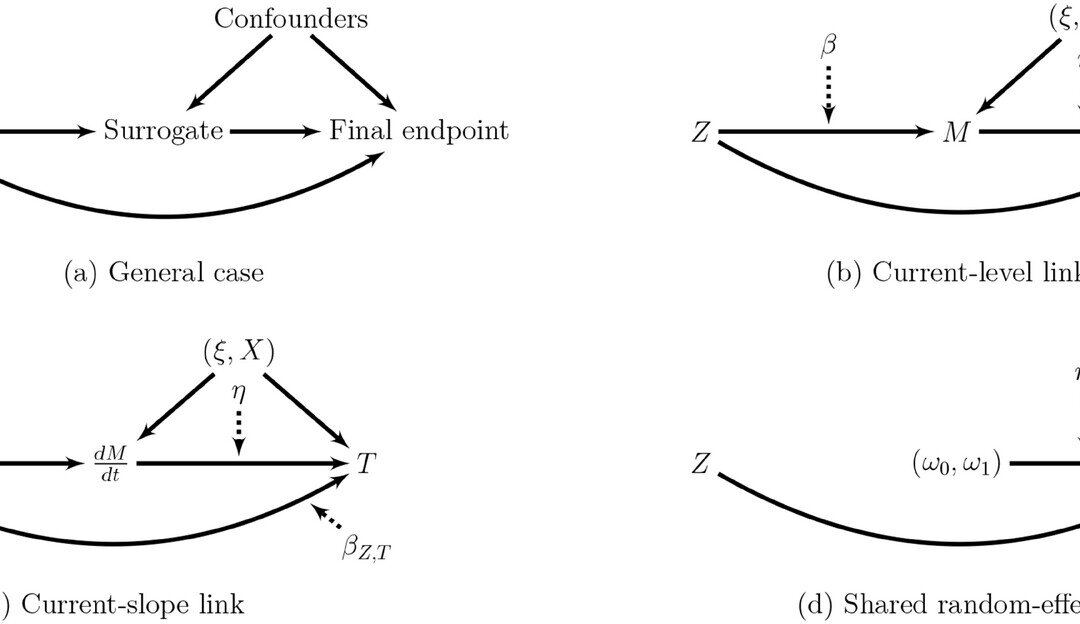
They looked at a real data application as well which was a multicenter study on locally advanced prostate cancer and its advancement overtime as a potential surrogate. The centers or institutions were used as clustering units. They followed time to occurrence of a local progression, distant metastasis, a biochemical failure, or death, whichever occurred first. For the function of time, they used different functions and then setup their joint model accordingly as they had defined in their methods but now for this dataset. They had f(t) = (1,f1(t),f2(t))’ so they estimated two models, a current-level link function and a current-slope link. For the latter model for purposes of mediation they had to add in an interaction term between treatment and f2(t) and for the evolution of PTE(t) they used 3 timepoints. They didn’t find any significant mediating effect of the slope but they did with the current-level link function.
An advantage of their approach is that it can be applied to meta-analytic data and not just focused on single center data. For the trajectory over time they used a mixed model but other approaches based on a mechanistic model have been proposed in the context of the joint modeling. However for the mediation model, the association term in the link function needs to depend upon treatment. They recommend that the interpretation of the PTE be done after looking at the direct and indirect effects separately. They also suggested combining the two link functions as surrogates of the survival endpoint, but this could complicate the computation. They have developed an R function for this: longiPenal in their frailtypack library.
Written by,
Usha Govindarajulu
Keywords: survival analysis, mediation, longitudinal, random effects, direct effect, indirect effect, frailtypack, R software, heterogeneity
References:
Coent QL, Legrand C, Dignam JJ, and Rondeau V (2025) “Validation of a Longitudinal Marker as a Surrogate Using Mediation Analysis and Joint Modeling: Evolution of the PSA as a Surrogate of the Disease-Free Survival” Biometrical Journal.
https://doi.org/10.1002/bimj.70064
https://onlinelibrary.wiley.com/cms/asset/ff5bd225-bdb3-4ec4-8270-eb2e04dd2c9c/bimj70064-fig-0001-m.jpg