
October 7, 2026
The authors discuss in their short communication whether the hazard function should be used for causal inference in tie-to-event studies and they consider three different potential outcome frameworks (by Rubin, Robins, and Pearl) respectively as well as the single-world intervention graph in order to show mathematically that the hazard function has causal interpretations under all three frameworks. Hernan (2010) seems to have first called out the hazard ratio (HR) as biased and that a time-varying one has no causal interpretation. He cited the Women’s Health Initiative (WHI) where HR was used as the primary measure of treatment effect. He referred to their hormone therapy trial among postmenopausal women with a uterus with randomized estrogen plus progestin compared to placebo. The trial had been stopped early due to significant elevation in breast cancer risk in the combined hormone therapy arm. The selection bias was formalized as a collider bias when conditioning on a risk set in the presence of heterogeneity. Prentice and Aragaki (2022) went on to defend the hazard ratio and Cox regression that the HR could capture empirical changes in current risk over time.
Aalen et al. (2015), Hernán (2010), and Martinussen et al. (2020) concluded that the HR cannot be causally interpreted because the risk sets, that is, the conditioning sets comprised of the subsets of individuals who have not previously failed, differ beyond the first event time. Also in referring to the WHI trial with cardiovascular outcome (Manson et al. 2004), which also provided estimated HR’s during each year of follow-up, Hernán (2010) stated that “differential selection of less susceptible women over time was the built-in selection bias of period-specific hazard ratios.”
Aalen et al. (2015) Claimed That the Selection Bias Results From a Collider Bias. Martinussen et al. (2020) Proposed an Alternative “Causal” HR. They first confirm that a time-fixed hazard ratio 𝛽 delivers causal interpretation. Prentice and Aragaki (2020) (Figure 1) showed that an estimated averaged hazard ratio (Kalbfleisch and Prentice, 1981, AHR) over time starting from 1 year post-randomization through year 16 is more sensitive to detecting early treatment effect than, for example, estimates of cumulative quantities, like the restricted mean survival time (RMST). In particular, the AHR estimate for coronary heart disease showed an early significant elevation during the first 6 years from randomization, while the RMST did not show any such difference. For breast cancer, the AHR estimator was elevated starting about year 6 from randomization and remained significant thereafter, while a reduction in RMST did not show significance until 12 years post-randomization.
They give their core defense to demonstrate that the time-varying hazard ratio 𝛽(𝑡) preserves full causal legitimacy across all three foundational definitions detailed in Section 1.1.
(a)Rubin’s framework
As they pointed out, under Rubin’s strict point-level identicality condition, critics argue that their raw comparison for the HR fails to yield a causal parameter because of the target subsets set1 ={𝑖:𝑌1,𝑖(𝑡)=1} and set0 ={𝑖:𝑌0,𝑖(𝑡)=1} differ over time. They claim to have countered this by emphasizing that the instantaneous hazard profile can be entirely recovered via a transformation of the baseline marginal counterfactual survival functions.
(b)Robin’s framework
They pointed out that since James Robins’ framework explicitly defines population causal effects as contrasts over any valid functional of the isolated marginal distributions of counterfactual outcomes, the time-varying hazard trajectory 𝛽(𝑡) directly qualifies as a legitimate causal estimand.
(c ) Pearl’s framework
Regarding evaluating a contrast between treatment groups by taking the ratio of these distinct counterfactual hazard curves yields a completely legitimate causal interpretation under Judea Pearl’s structural causal framework. They emphasized that only the entire time-varying parameter 𝛽(𝑡) across all time points has a causal interpretation, instead of at a single point.
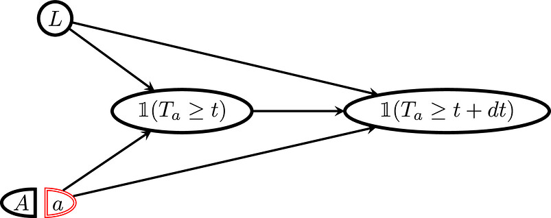
They then bring up a point of confusion in Hernán (2010) is about “less susceptible women.”, which they say this has been well understood in the literature as unobserved heterogeneity, referred to as frailty, since at least as early as Lancaster (1979). They further went on to say that in other words, the “differential selection … over time” is due to the existence of unobserved heterogeneity, also referred to as over-dispersion, and not “period-specific hazard ratios” as speculated in Hernán (2010). They then showed a SWIG (single-world intervention graph) to demonstrate why the counterfactual risk does not suffer from collider bias. Consequently, there is no active path originating from 𝐴 that collides at 𝑌𝑎(𝑡) with the unobserved baseline heterogeneity 𝐿. They also further argued that the causal hazard ratio is not satisfactory.
According to the authors, the WHI examples described in Prentice and Aragaki (2022) provided convincing applications of hazard ratio in the past several decades in medical research. Accordig to them, the early stopping of both of the WHI trials has to do with the fact that, without making the proportional hazards assumption, the average hazard ratio is more sensitive to detecting early differences than the alternative restricted mean survival time, for example (Prentice and Aragaki (2022).
All in all, this is a very complicated defense of the hazard ratio and their use of the WHI study to explain why the hazard ratio was fine has still not been enough justification or legitimacy per this article. Also, their justification of the HR per each approach (Rubin, Robin, Pearl) is vague and not given enough proof for each. Basically, this article is not enough of a defense of the HR.
Written by,
Usha Govindarajulu, MS PhD
Keywords: survival analysis, hazard ratio, proportional hazard assumption,
References:
Aalen, O. O., R. J. Cook, and K. Røysland. 2015. “Does Cox Analysis of a Randomized Survival Study Yield a Causal Treatment Effect?” Lifetime Data Analysis 21, no. 4: 579–593.
Hernán, M. A., and J. M. Robins. 2020. Causal Inference: What If. CRC Press.
Kalbfleisch, J. D., and R. L. Prentice. 1981. “Estimation of the Average Hazard Ratio.” Biometrika 68: 105–112.
Lancaster, T. 1979. “Econometric Methods for the Duration of Unemployment.” Econometrica 47, no. 4: 939–956.
Manson, J. E., J. Hsia, K. C. Johnson, et al. 2004. “Estrogen Plus Progestin and the Risk of Coronary Heart Disease.” New England Journal of Medicine 349, no. 6: 523–534.
Martinussen, T., S. Vansteelandt, and P. K. Andersen. 2020. “Subtleties in the Interpretation of Hazard Contrasts.” Lifetime Data Analysis 26, no. 4: 833–855.
Prentice, R. L., and A. K. Aragaki. 2022. “Intention-to-Treat Comparisons in Randomized Trials.” Statistical Science 37, no. 3: 380–393.
Ying A and Xu R (2026) “On Defense of the Hazard Ratio” Biometrical Journal . 68(5): e70187
https://doi.org/10.1002/bimj.70187
https://onlinelibrary.wiley.com/cms/asset/f15fe03c-f68c-4be1-96db-667d2de73ba4/bimj70187-fig-0002-m.jpg